Detection of gene set spatial patterns and expression gradients in CosMx-SMI

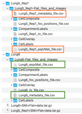
The package spatialGE can be used to detect spatial patterns in gene expression at the gene and gene set level. Data from multiple spatial transcriptomics platforms can be analyzed, as long as gene expression counts per spot or cell are associated with spatial coordinates of those spots/cells. The spatialGE package is also compatible with outputs from the Visium workflow (i.e., Space Ranger) or the CosMx-SMI spatial single-cell platform.

In this tutorial, the functions STenrich, STclust, and STgradient will be used to test for spatial gene set enrichment and genes showing expression gradients on a CosMx-SMI data set from Non-Small Cell Lung Cancer (NSCLC).

How is spatialGE installed?

The spatialGE repository is available at GitHub and can be installed via devtools. To install devtools (in case it is not already installed in your R), please run the following code:

if("devtools" %in% rownames(installed.packages()) == FALSE){
  install.packages("devtools")
}

After making sure devtools is installed, proceed to install spatialGE:

# devtools::install_github("fridleylab/spatialGE")

Spatial gene set enrichment and expression gradients in non-small cell lung cancer (NSCLC)

The CosMx-SMI platform generates single-cell level gene expression with associated x and y locations of the cells where measurements were taken. For the data set used in this tutorial, RNA counts were measured for 960 genes in about 800K cells. The data was generated from eight tissue slices, with counts obtained for a series of Fields of Vision (FOVs) within each slice. However, in this tutorial, the data set has been subset to 6 FOVs originating from two of the slices.

The complete data set can be downloaded from the links below. It is also likely that registration in the website is necessary in order to download the data set.

The data from the 6 FOVs used in this tutorial is available at the spatialGE_Data GitHub repository. Data will be downloaded and deposited in a temporary directory. However, the download path can be changed within the following code block:

nsclc_tmp = tempdir()
unlink(nsclc_tmp, recursive=TRUE)
dir.create(nsclc_tmp)
download.file('https://github.com/FridleyLab/spatialGE_Data/raw/refs/heads/main/nanostring_nsclc.zip?download=', 
              destfile=paste0(nsclc_tmp, '/', 'nanostring_nsclc.zip'), mode='wb')
zip_tmp = list.files(nsclc_tmp, pattern='nanostring_nsclc.zip$', full.names=TRUE)
unzip(zipfile=zip_tmp, exdir=nsclc_tmp)

Data for each tissue slice is stored in separate folders. The structure of the files is shown below:

The key files are shown enclosed in orange (Lung 5-1) and green (Lung 6) boxes. The “_exprMat_file.csv” file of each sample contains the gene counts. The “_metadata_file.csv” contains the cell x, y coordinates for each sample. Optionally, the “CellComposite” folder contains images that can be imported into the STlist (details later in this tutorial).

From the temporary directory, the file paths to be passed to the STlist function are:

# Find expression and coordinates files within the temporary folder
exprmats <- c(
  paste0(nsclc_tmp, '/nanostring_nsclc/Lung5_Rep1-Flat_files_and_images/Lung5_Rep1_exprMat_file_SUBSET.csv'),
  paste0(nsclc_tmp, '/nanostring_nsclc/Lung6-Flat_files_and_images/Lung6_exprMat_file_SUBSET.csv')
)
metas <- c(
  paste0(nsclc_tmp, '/nanostring_nsclc/Lung5_Rep1-Flat_files_and_images/Lung5_Rep1_metadata_file_SUBSET.csv'),
  paste0(nsclc_tmp, '/nanostring_nsclc/Lung6-Flat_files_and_images/Lung6_metadata_file_SUBSET.csv')
)

Now, that the data is ready, load the spatialGE package:

library('spatialGE')

Creating an STList (Spatial Transcriptomics List)

The starting point of a spatialGE analysis is the creation of an STlist (S4 class object), which stores raw and processed data. The STlist is created with the function STlist, which can take data in multiple formats (see here for more info or type ?STlist in the R console).

To load the files into an STlist, please use these commands:

lung <- STlist(rnacounts=exprmats, 
               spotcoords=metas, 
               samples=c('Lung5_Rep1', 'Lung6'), cores=2)
#> Found CosMx-SMI data
#> Found 2 CosMx-SMI samples
#>  Data read completed
#> Matching gene expression and coordinate data...
#> Converting counts to sparse matrices
#> Completed STlist!

To obtain count statistics, the summarize_STlist function can be used:

summ_df = summarize_STlist(lung)
summ_df
#> # A tibble: 6 × 9
#>   sample_name     spotscells genes min_counts_per_spotc…¹ mean_counts_per_spot…²
#>   <chr>                <int> <int>                  <dbl>                  <dbl>
#> 1 Lung5_Rep1_fov…       3744   980                      2                   326.
#> 2 Lung5_Rep1_fov…       5272   980                      0                   328.
#> 3 Lung5_Rep1_fov…       3946   980                      2                   367.
#> 4 Lung6_fov_4           3310   980                      1                   304.
#> 5 Lung6_fov_6           3325   980                      0                   523.
#> 6 Lung6_fov_7           3477   980                      0                   312.
#> # ℹ abbreviated names: ¹min_counts_per_spotcell, ²mean_counts_per_spotcell
#> # ℹ 4 more variables: max_counts_per_spotcell <dbl>,
#> #   min_genes_per_spotcell <int>, mean_genes_per_spotcell <dbl>,
#> #   max_genes_per_spotcell <int>

Some cells have zero counts. We can look at the distribution of counts per cell for the first five and last five FOVs using the distribution_plots function:

cp <- distribution_plots(lung, plot_type='violin', plot_meta='total_counts', samples=c(1:5, 56:60))
#> Sample NA does not contain total_counts.
#> Sample NA does not contain total_counts.
#> Sample NA does not contain total_counts.
#> Sample NA does not contain total_counts.
#> Sample NA does not contain total_counts.
cp[['total_counts']]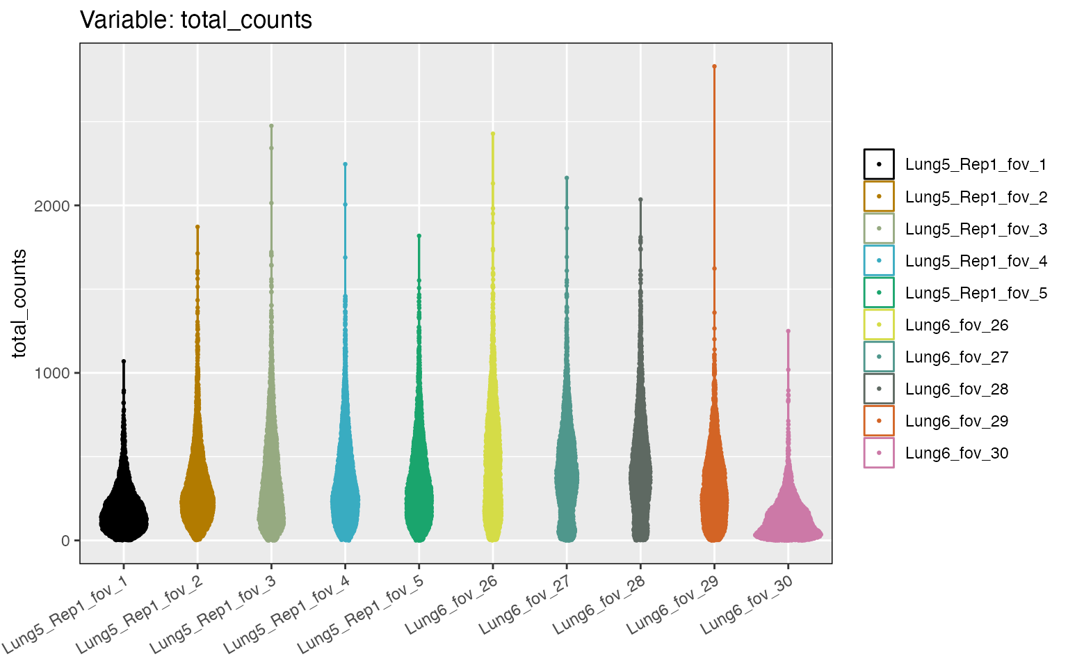

Cells with zero counts, can be removed using the filter_data function. The function can also be used to remove all counts from specific genes. This option is useful in this case, as CosMx-SMI panels include negative probe genes. While the negative probes can be used in normalization of counts, in this tutorial those genes will be removed. Negative probes in CosMx-SMI begin with the token “NegPrb”:

lung <- filter_data(lung, spot_minreads=20, rm_genes_expr='^NegPrb')

Transformation of spatially-resolved transcriptomics data

The function transform_data allows data transformation using one of two possible options. The first options applies log-transformation to the counts, after library size normalization performed on each sample separately. The second option applies variance-stabilizing transformation (SCT; Hafemeister and Satija (2019)), which is a method increasingly used in single-cell and spatial transcriptomics studies. To apply SCT transformation, use the following command:

lung <- transform_data(lung, method='sct', cores=2)

Detecting gene sets with spatial aggregation patterns

An important part of gene expression analysis is the use of gene sets to make inferences about the functional significance of changes in expression. Normally, this is achieved by conducting a Gene Set Enrichment Analysis (GSEA). While GSEA can be completed in a similar fashion to scRNA-seq, it is possible with the STenrich function to test for gene sets that show spatial non-uniform enrichment. In other words, STenrich tests whether expression of a gene set is concentrated in one or few areas of the tissue.

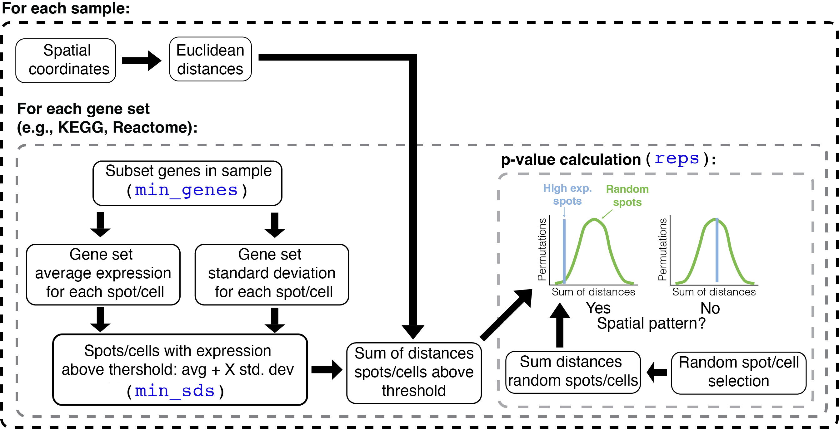
The algorithm in STenrich is depicted in the following diagram:

The STenrich function is a modification of the method proposed by Hunter et al. (2021). The steps in this modified version are as follows: First, Euclidean distances are calculated among all spots/cells. Then, the gene expression of the sample is subset to the genes within the gene set being tested. If too few genes are left after subset (min_genes), then the gene set is omitted for that sample. The average expression and standard deviation of those genes is calculated for each spot/cell. Next, spots/cells with gene set expression above the average gene set expression across all spots/cells are identified. The threshold to define these high gene set expression spots is defined by the average gene set expression plus a number min_sds of standard deviations. The sum of the Euclidean distances between the high expression spots/cells is calculated.

The next step involves a permutation process, in which a null distribution is generated in order to test if the (sum of) distances among high expression spots are smaller than expected. To that end, a random sample of spots/cells (regardless of expression) is selected. The random sample has the same size as the number of high expression spots/cells. Then, the sum of distances among the randomly sampled spots/cells is calculated. The random selection is repeated as many times as requested (`reps``). Finally, a p-value is calculated by noting how many times the sum of random distances was higher than the sum of distances among high expression spots/cells. If the sum of random distances was most of the times higher than the sum of distances among high expression spots/cells, then the null hypothesis of no spatial aggregation is rejected (i.e., spots/cells with high gene set expression are more aggregated than expected by chance).

A few important notes about the algorithm to consider:

Notice that the metric of enrichment is currently the average expression of the genes in a set within each ROI/spot/cell. Better metrics of gene set enrichment are available and will be soon available to use instead of average.
Special attention should be paid to the reference genome used to annotate gene counts. The annotation of transcripts precedes any analysis in spatialGE. Nevertheless, if transcripts are annotated with a mouse genome (or other species), the user should use the appropriate gene set database, as gene names will likely not match to a gene set database with human gene names. Furthermore, but not less important, there might be problems with gene homology.
The more permutations are requested, the longer the execution, but p-value estimates are more accurate.
By increasing the number of standard deviations, fewer spots/cells are selected as “high expression” (stringent analysis), however, it becomes more challenging to detect gene sets that show evidence of spatial aggregation. Values between 1 to 2 standard deviations are likely suitable for most studies.
By adjusting the minimum number of spots (min_spots), the user has some rough control over the size of the structures to be studied. For example, small immune infiltrates could be detected with smaller number of minimum spots. Conversely, if tissue domain-level differences are sought, then a larger Minimum number of spots should be set.
Take note of the random seed number used for the test (Seed number parameter), in case you need to generate the same results later. Nevertheless, running the analysis several times with different seed numbers is advisable to check for consistency.

The first step to run STenrich is to obtain a list of gene sets. Here, the msigdbr package will be used to obtain HALLMARK gene sets:

# Load msigdbr
library('msigdbr')

# Get HALLMARK gene sets
gene_sets <- msigdbr(species='Homo sapiens')
# Select the appropriate column depending on the msigdbr version
gs_column <- grep('gs_cat|gs_collection', colnames(gene_sets), value=T)[1]
gene_sets <- gene_sets[gene_sets[[gs_column]] == "H", ]

# Convert gene set dataframe to list
# The result is a named list. The names of the list are the names of each gene set
# The contents of each list element are the gene names within each gene set
gene_sets <- split(x=gene_sets[['gene_symbol']], f=gene_sets[['gs_name']])

For the purpose of this example, we will only test “signaling” pathways:

gene_sets = gene_sets[grep('SIGNALING', names(gene_sets))]

Please keep in mind that it is assumed that HUGO gene names are used. For CosMx-SMI and Visium, normally HUGO names are provided. If spatial transcriptomics data from a non-human species is used, the appropriate database should be used. Otherwise, spatialGE will not be able to identify genes within the gene set.

The STenrich function can now be used. For this analysis, 1000 replicates (reps=1000) will be used to generate the null distribution. In addition, for a gene set to be considered as highly expressed in cell, it should be expressed at least over the average expression plus 1.5 standard deviations (num_sds=1.5). Gene sets with less than five genes in the sample (min_genes=5) and gene sets with less than 10 highly expressed cells (min_units=10) will not be tested. Notice a seed was set (seed=12345), which critical for replication of the results in the future.

stenrich_df <- STenrich(lung, gene_sets=gene_sets, 
                        reps=1000, 
                        num_sds=1.5, 
                        min_genes=5,
                        min_units=10, 
                        seed=12345, cores=2) 
#> Running STenrich...
#>  Calculating average gene set expression...
#> STenrich completed in 0.41 min.

The result of the function is a list of data frames, with one data frame per samples (FOV in this case). For example, this is the data frame for the first FOV in the STlist:

head(stenrich_df$Lung5_Rep1_fov_1)
#>          sample_name                         gene_set size_test size_gene_set
#> 15 Lung5_Rep1_fov_11 HALLMARK_IL6_JAK_STAT3_SIGNALING        58           103
#> 27 Lung5_Rep1_fov_11       HALLMARK_KRAS_SIGNALING_UP        55           220
#> 57 Lung5_Rep1_fov_11 HALLMARK_TNFA_SIGNALING_VIA_NFKB        76           228
#> 9  Lung5_Rep1_fov_11     HALLMARK_IL2_STAT5_SIGNALING        58           216
#> 21 Lung5_Rep1_fov_11       HALLMARK_KRAS_SIGNALING_DN        20           220
#> 33 Lung5_Rep1_fov_11        HALLMARK_MTORC1_SIGNALING        13           211
#>    prop_size_test p_value adj_p_value
#> 15          0.563   0.000      0.0000
#> 27          0.250   0.004      0.0200
#> 57          0.333   0.009      0.0300
#> 9           0.269   0.213      0.5325
#> 21          0.091   0.295      0.5900
#> 33          0.062   1.000      1.0000

Each row represents a test for the null hypothesis of no spatial aggregation in the expression of the set in the “gene_set” column. The column “size_test” is the number of genes of a gene set that were present in the FOV. The larger this number the better, as it indicates a better representation of the gene set in the sample. The “adj_p_value” is the multiple test adjusted p-value, which is the value used to decide if a gene set shows significant indications of a spatial pattern (adj_p_value < 0.05).

With a few lines of code, a visual summary can be generated that presents the gene sets with adj_p_value < 0.05 across FOVs for each tissue slide:

# Load tidyverse for data frame manipulation
library('tidyverse')

# Combine all samples in a single data frame
# Subset to gene sets showing significant evidence of spatial pattern (adj_p_value < 0.05) and
# proportion higher or equal than 0.3 of genes from a gene set present in sample 
res <- bind_rows(stenrich_df) %>%
  mutate(prop_gene_set=size_test/size_gene_set) %>%
  filter(prop_gene_set >= 0.3 & adj_p_value < 0.05) %>%
  mutate(slide=str_extract(sample_name, "Lung5_Rep1|Lung6")) %>%
  select(slide, gene_set) %>%
  mutate(gene_set=str_replace(gene_set, 'HALLMARK_', ''))

# Generate barplot showing the number of FOVs with siginificant evidence of spatial
# patterns for each tissue slide
ggplot(res) + 
  geom_bar(aes(x=gene_set)) +
  xlab(NULL) +
  theme(axis.text.x=element_text(angle=70, vjust=1, hjust=1)) +
  facet_wrap(~slide)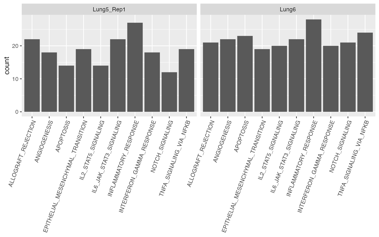

The “NOTCH signaling” pathway showed spatial patterns less frequently in the slide “Lung5_Rep1” compared to “Lung6”. With the function STplot, the average gene set expression for this pathway can be plotted. First, FOVs with and without NOTCH signaling spatial patterns will be identified from “Lung5_Rep1” and “Lung6” respectively.

bind_rows(stenrich_df) %>%
  mutate(prop_gene_set=size_test/size_gene_set) %>%
  filter(prop_gene_set >= 0.3 & adj_p_value >= 0.05) %>%
  arrange(desc(prop_gene_set), desc(adj_p_value)) %>%
  filter(gene_set == 'HALLMARK_NOTCH_SIGNALING') %>%
  filter(str_detect(sample_name, "Lung5_Rep1")) %>%
  slice_head(n=3)
#>         sample_name                 gene_set size_test size_gene_set
#> 1 Lung5_Rep1_fov_11 HALLMARK_NOTCH_SIGNALING        13            34
#> 2  Lung5_Rep1_fov_2 HALLMARK_NOTCH_SIGNALING        13            34
#> 3  Lung5_Rep1_fov_6 HALLMARK_NOTCH_SIGNALING        13            34
#>   prop_size_test p_value adj_p_value prop_gene_set
#> 1          0.382   0.989       1.000     0.3823529
#> 2          0.382   0.981       0.981     0.3823529
#> 3          0.382   0.858       0.977     0.3823529

bind_rows(stenrich_df) %>%
  mutate(prop_gene_set=size_test/size_gene_set) %>%
  filter(prop_gene_set >= 0.3 & adj_p_value < 0.05) %>%
  arrange(desc(prop_gene_set), adj_p_value) %>%
  filter(gene_set == 'HALLMARK_NOTCH_SIGNALING') %>%
  filter(str_detect(sample_name, "Lung6")) %>%
  slice_head(n=3)
#>   sample_name                 gene_set size_test size_gene_set prop_size_test
#> 1 Lung6_fov_4 HALLMARK_NOTCH_SIGNALING        13            34          0.382
#> 2 Lung6_fov_6 HALLMARK_NOTCH_SIGNALING        13            34          0.382
#> 3 Lung6_fov_7 HALLMARK_NOTCH_SIGNALING        13            34          0.382
#>   p_value adj_p_value prop_gene_set
#> 1   0.000 0.000000000     0.3823529
#> 2   0.000 0.000000000     0.3823529
#> 3   0.001 0.001666667     0.3823529

Plots can be generated like so:

qp <- STplot(lung, genes=gene_sets[names(gene_sets) == 'HALLMARK_NOTCH_SIGNALING'], 
             samples=c('Lung5_Rep1_fov_2', 'Lung5_Rep1_fov_6', 'Lung5_Rep1_fov_11',
                       'Lung6_fov_4', 'Lung6_fov_6', 'Lung6_fov_7'),
             color_pal='YlOrBr')

ggpubr::ggarrange(plotlist=qp, ncol=3, nrow=2, common.legend=TRUE)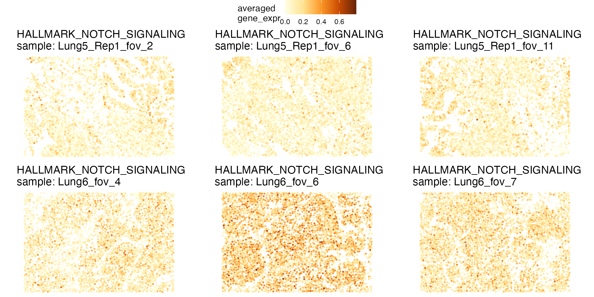

Although expression of the NOTCH signaling pathway is higher overall in “Lung6”, the expression is not uniform, but rather is arranged in patterns within each FOV. Conversely, cells in FOVs of “Lung5_Rep1” that show high expression of the NOTCH signaling pathway are scattered across the tissue.

Since this expression of this pathway has been identified as spatially aggregated, it might be of interest to know if there is correspondence of NOTCH signaling with tissue domains. With the STclust function, tissue domains can be identified.

lung <- STclust(lung, ws=0.02, ks='dtc', cores=2)
#> STclust started...
#> Updating STlist with results...
#> STclust completed in 0.41 min.

Optinally, if tissue images are available for some or all the FOVs, users can upload those to the STlist for display next to the other plot types available in spatialGE. Users can upload an entire folder of images to the STlist, as long as image files have the same names as the FOVs within the STlist (e.g., “Lung5_Rep1_fov_2”, “Lung6_fov_4”, etc). Keep in mind, however, this will increase the size of the STlist significantly, especially in CosMx experiments that usually contain many FOVs.

The multiplexed immunofluorescence images have been previously downloaded from the spatialGE_Data GitHub repository. The temporary folder created at the beggining of this tutorial will be used to generate the file paths to the folder containng the images. Importantly, the images need to be renamed according to the FOV name in the STlist. This renaming was already performed for the files in the spatialGE_Data GitHub repository. Here is an example of how the files were renamed from the original data set:

For tissue slice “Lung5_Rep1”, images were renamed from “CellComposite_F002.jpg”, “CellComposite_F006.jpg”, and “CellComposite_F011.jpg” to “Lung5_Rep1_fov_2.jpg”, “Lung5_Rep1_fov_6.jpg”, and “Lung5_Rep1_fov_11.jpg” respectively.
For tissue slice “Lung6”, images were renamed from “CellComposite_F004.jpg”, “CellComposite_F006.jpg”, and “CellComposite_F007.jpg” to “Lung6_fov_4.jpg”, “Lung6_fov_6.jpg”, and “Lung6_fov_7.jpg” respectively.

Now, upload the images to the STlist with the load_images function:

img_fp = paste0(nsclc_tmp, '/nanostring_nsclc/Lung5_Rep1-Flat_files_and_images/CellComposite')
lung <- load_images(lung, images=img_fp)
#> Image for sample Lung6_fov_4 was not found.
#> Image for sample Lung6_fov_6 was not found.
#> Image for sample Lung6_fov_7 was not found.

The images for slide “Lung6” were not found, which are in the corresponsing folder. The load_images function is ran again to add images from “Lung6”:

img_fp = paste0(nsclc_tmp, '/nanostring_nsclc/Lung6-Flat_files_and_images/CellComposite')
lung <- load_images(lung, images=img_fp)
#> Image for sample Lung5_Rep1_fov_2 was not found.
#> Image for sample Lung5_Rep1_fov_6 was not found.
#> Image for sample Lung5_Rep1_fov_11 was not found.

The function plot_image is used to generate the ggplot objects containing the images:

ti <- plot_image(lung)

The domains can be plotted with the STplot function too.

dom_p <- STplot(lung, ks='dtc', ws=0.02, deepSplit=FALSE,
                color_pal='discreterainbow')

ggpubr::ggarrange(dom_p$Lung5_Rep1_fov_2_stclust_spw0.02_dsplFalse,
                  ti$image_Lung5_Rep1_fov_2,
                  dom_p$Lung5_Rep1_fov_6_stclust_spw0.02_dsplFalse,
                  ti$image_Lung5_Rep1_fov_6,
                  dom_p$Lung5_Rep1_fov_11_stclust_spw0.02_dsplFalse,
                  ti$image_Lung5_Rep1_fov_11,
                  dom_p$Lung6_fov_4_stclust_spw0.02_dsplFalse,
                  ti$image_Lung6_fov_4,
                  dom_p$Lung6_fov_6_stclust_spw0.02_dsplFalse,
                  ti$image_Lung6_fov_6,
                  dom_p$Lung6_fov_7_stclust_spw0.02_dsplFalse,
                  ti$image_Lung6_fov_7,
                  ncol=4, nrow=3)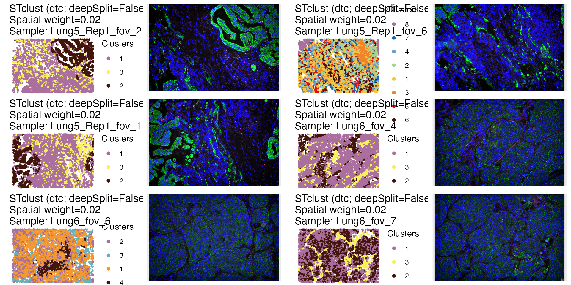


# If no tissue images are available:
# ggpubr::ggarrange(plotlist=dom_p, ncol=3, nrow=2)

Now, to identify the domains, differential gene expression can be performed:

deg <- STdiff(lung, w=0.02, k='dtc', deepSplit=FALSE, test_type='wilcoxon', cores=2)
#> Testing STclust assignment (w=0.02, dtc deepSplit=False)...
#>  Running Wilcoxon's tests...
#>  Completed Wilcoxon's tests (5.77 min).
#> STdiff completed in 5.77 min.

Then, the top 3 DE genes per cluster in the samples showing NOTCH signaling spatial patterns are identified:

bind_rows(deg) %>%
  filter(adj_p_val < 0.05 & abs(avg_log2fc > 0.05)) %>%
  filter(sample %in% c('Lung6_fov_4', 'Lung6_fov_6', 'Lung6_fov_7')) %>%
  group_by(sample, cluster_1) %>%
  slice_head(n=3)
#> # A tibble: 57 × 6
#> # Groups:   sample, cluster_1 [19]
#>    sample      gene     avg_log2fc cluster_1 wilcox_p_val adj_p_val
#>    <chr>       <chr>         <dbl> <chr>            <dbl>     <dbl>
#>  1 Lung6_fov_4 KRT15         0.895 1            7.13e-194 8.56e-191
#>  2 Lung6_fov_4 IL1R1         0.361 1            1.24e- 82 2.29e- 80
#>  3 Lung6_fov_4 KRT17         0.416 1            1.58e- 76 2.23e- 74
#>  4 Lung6_fov_4 H4C3          0.574 2            2.87e-105 8.12e-103
#>  5 Lung6_fov_4 HSP90AA1      0.473 2            4.61e- 94 1.05e- 91
#>  6 Lung6_fov_4 H2AZ1         0.424 2            1.37e- 87 2.74e- 85
#>  7 Lung6_fov_4 CD74          0.697 3            4.70e-226 2.26e-222
#>  8 Lung6_fov_4 HLA-DRB1      0.790 3            7.49e-211 1.20e-207
#>  9 Lung6_fov_4 VIM           0.533 3            2.84e-180 2.72e-177
#> 10 Lung6_fov_4 KRT13         1.06  4            1.59e-131 7.62e-129
#> # ℹ 47 more rows

Expression of KRT genes in domains 1 and 2 of FOVs “Lung6_fov_4” and “Lung6_fov_7”, and domains 2 and 4 of “Lung6_fov_6” are indicative of tumor cells. In those domains (with the exception of 4 in “Lung6_fov_6”), there seems to be an overlap with the areas of of NOTCH signaling, which indicates that in slide “Lung6”, the tumor compartment is spatially enriched for NOTCH signaling.

Identifcation of genes presenting expression spatial gradients

Since the tumor areas have been visually identified, it is possible now to ascertain which genes show expression that varies with distance within the tumor compartment. In the FOVs “Lung6_fov_4”, “Lung6_fov_7”, and “Lung6_fov_6”, the domain 3 seems to be surrounding the tumor compartment. Hence, domain 3 will be used as reference domain to test for genes for which expression increases or decreases with distance from domain 3. 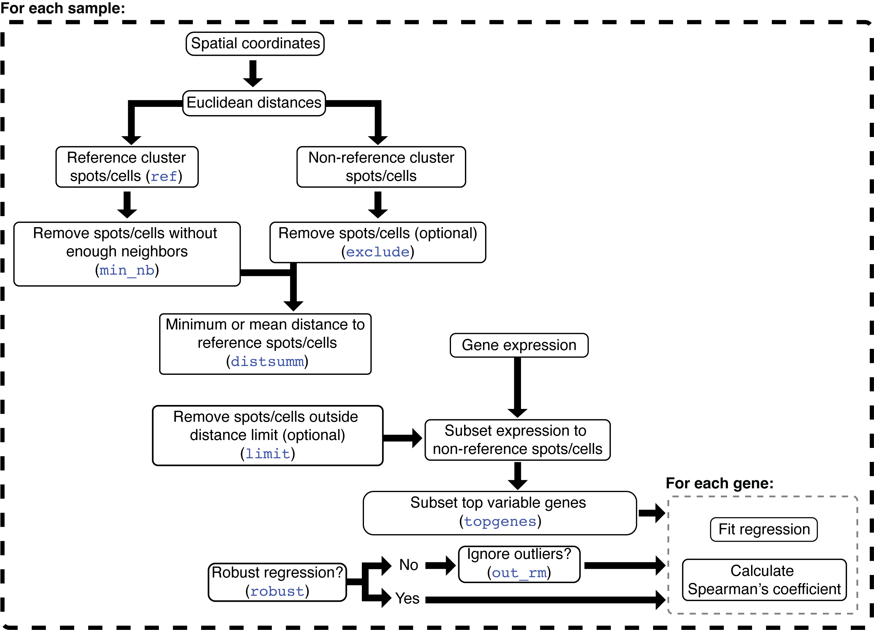This test is performed by the STgradient function. The following diagram depicts the STgradient algorithm:

In STgradient, the spatial coordinates are used to calculate Euclidean distances of each cell to each of the other cells. The reference domain is the domain from which the distances will be calculated (domain 3 in this case). The non-reference domain(s) are the domain(s) on which the user wants to study gradients. Next, removes isolated spots/cells in the reference domain (i.e., have a number of immediate neighbors smaller than parameter min_nb). The min_nb parameter intends to reduce the effects of small “pockets” of the reference domain on the correlation coefficient. At this point, either the minimum or average distance of each non-reference cell to each reference cell is calculated (distsumm). The minimum distance is easier to interpret, however, it is more sensitive to highly fragmented reference domains. On the other hand, the interpretability of the average distance is not as easy as the minimum distance, but it might detect in a better way the gradients when the reference domain is distributed across the sample. Next, the gene expression data is subset to the non-reference spots/cells, and the top variable genes (topgenes) are selected. Results will be produced only for those genes. Depending on the user’s selection, the ordinary least squares (OLS) or robust regression is used to calculate the slope of the regression line between the minimum/average distance and the expression of a gene. If OLS was selected, users might opt to remove outliers via the interquartile method. Finally, the Spearman’s coefficient is calculated in addition to the regression line coefficient. The slope indicates the direction of the correlation. If positive, the gene expression tends to be higher when farther from the reference domain. If negative, gene expression is higher when closer to the reference domain. The interpretation of the sign for the Spearman’s coefficient is similar, however its magnitude indicates how strong the correlation is between gene expression and distance to the reference domain.

The STgradient function can be executed with these commands, in order to test for gradients within the tumor compartment. First, it is necessary to find the name of the column in lung_subset@spatial_meta containing the domain assigments:

colnames(lung@spatial_meta$Lung5_Rep1_fov_2)
#> [1] "libname"                   "xpos"                     
#> [3] "ypos"                      "total_counts"             
#> [5] "total_genes"               "stclust_spw0.02_dsplFalse"

The name of the column is stclust_spw0.02_dsplFalse (STclust results using spatial weight of 0.02 and DynamicTreeCuts with no deepSplit). This name is used in the annot argument of STgradient:

stg <- STgradient(lung, 
                  topgenes=1000, 
                  annot='stclust_spw0.02_dsplFalse',
                  ref=3,
                  samples=c('Lung6_fov_4', 'Lung6_fov_6', 'Lung6_fov_7'), 
                  distsumm='min', 
                  robust=TRUE, cores=2)
#> STgradient completed in 0.1 min.

Here are the first few rows of the STgradient result for sample “Lung6_fov_4”:

head(stg$Lung6_fov_4)
#> # A tibble: 6 × 8
#>   sample_name gene   min_lm_coef min_lm_pval min_spearman_r min_spearman_r_pval
#>   <chr>       <chr>        <dbl>       <dbl>          <dbl>               <dbl>
#> 1 Lung6_fov_4 HLA-B    -0.000213    2.63e-28         -0.208            2.73e-28
#> 2 Lung6_fov_4 S100A2    0.000222    8.32e-31          0.208            1.75e-28
#> 3 Lung6_fov_4 EGFR      0.000133    3.19e-18          0.200            2.36e-26
#> 4 Lung6_fov_4 MT1X      0.000132    2.75e-17          0.192            2.82e-24
#> 5 Lung6_fov_4 KRT6A     0.000231    2.47e-29          0.180            1.43e-21
#> 6 Lung6_fov_4 GPNMB     0.000125    6.22e-10          0.164            4.94e-18
#> # ℹ 2 more variables: min_spearman_r_pval_adj <dbl>, min_pval_comment <chr>

The key columns to look ar are min_spearman_r and min_spearman_r_pval_adj. Now, to find genes with significant spatial gradients across the three samples, these commands can be used:

bind_rows(stg) %>%
  arrange(desc(abs(min_spearman_r))) %>%
  group_by(sample_name) %>%
  slice_head(n=5) %>%
  ungroup() %>%
  arrange(gene)
#> # A tibble: 10 × 8
#>    sample_name gene   min_lm_coef min_lm_pval min_spearman_r min_spearman_r_pval
#>    <chr>       <chr>        <dbl>       <dbl>          <dbl>               <dbl>
#>  1 Lung6_fov_4 EGFR     0.000133     3.19e-18          0.200            2.36e-26
#>  2 Lung6_fov_6 FOS     -0.0000627    3.86e-23         -0.201            1.44e-26
#>  3 Lung6_fov_4 HLA-B   -0.000213     2.63e-28         -0.208            2.73e-28
#>  4 Lung6_fov_6 HSP90…   0.000112     6.96e-29          0.216            9.82e-31
#>  5 Lung6_fov_4 KRT6A    0.000231     2.47e-29          0.180            1.43e-21
#>  6 Lung6_fov_6 KRT6B   -0.0000891    1.91e-19         -0.180            9.61e-22
#>  7 Lung6_fov_4 MT1X     0.000132     2.75e-17          0.192            2.82e-24
#>  8 Lung6_fov_6 MT1X    -0.000181     2.52e-46         -0.285            6.02e-53
#>  9 Lung6_fov_6 NTRK2    0.000128     1.06e-32          0.231            7.62e-35
#> 10 Lung6_fov_4 S100A2   0.000222     8.32e-31          0.208            1.75e-28
#> # ℹ 2 more variables: min_spearman_r_pval_adj <dbl>, min_pval_comment <chr>

It can be seen from these results that multiple keratin genes show spatial gradients, all of them with negative Spearman’s coefficients (cells close to domain 3 tend to have higher keratin expression). Other such HLA-B and NDRG1 have higher expression in cells far from domain 3:

qp2 <- STplot(lung, genes=c('KRT6A', 'HLA-B'), samples='Lung6_fov_4', color_pal='YlOrBr')
ggpubr::ggarrange(plotlist=qp2, common.legend=TRUE)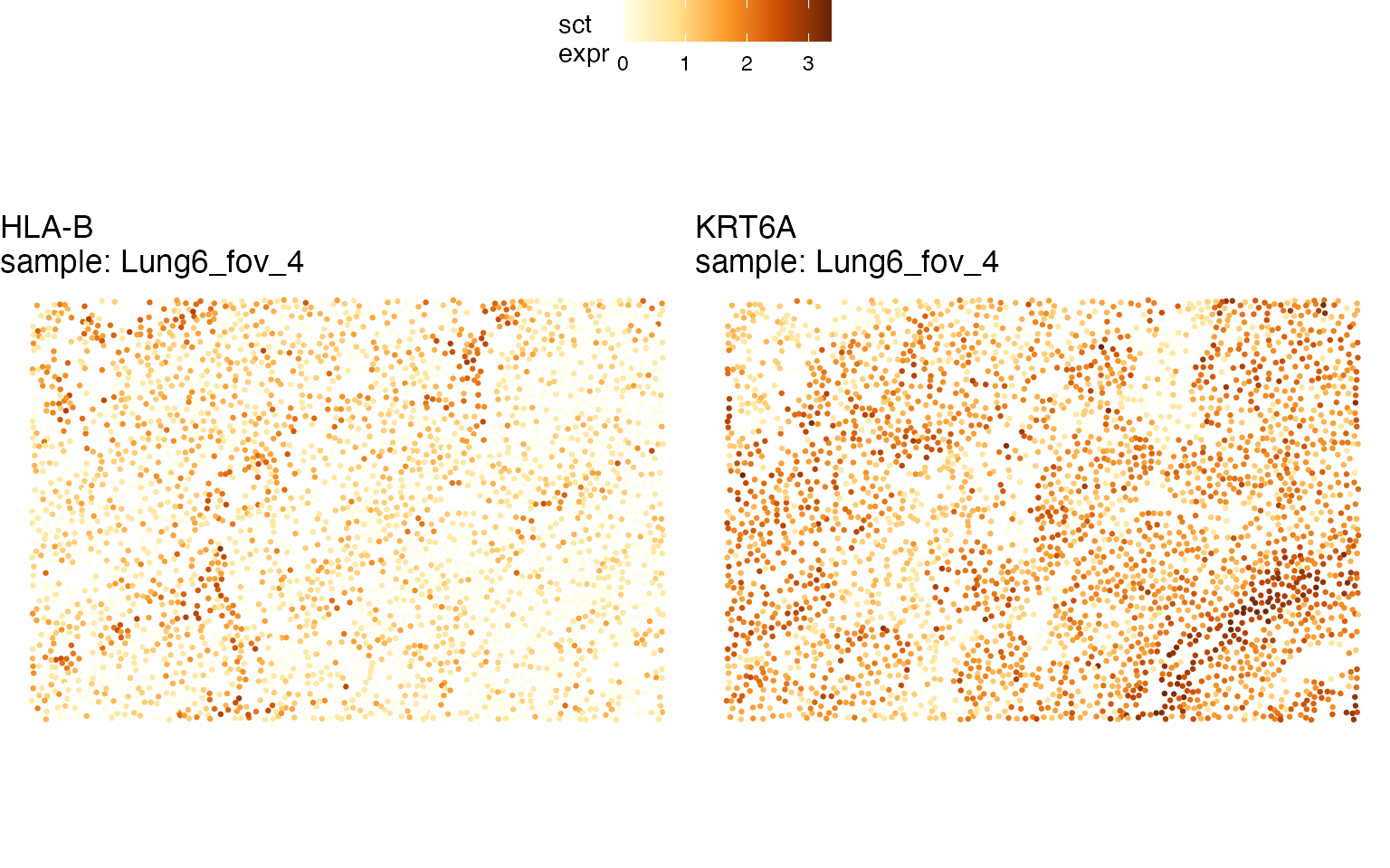

Here are the results for genes within the NOTCH signaling pathway:

bind_rows(stg) %>%
  arrange(desc(abs(min_spearman_r))) %>%
  filter(gene %in% gene_sets[['HALLMARK_NOTCH_SIGNALING']]) %>%
  filter(min_spearman_r_pval_adj < 0.05)
#> # A tibble: 3 × 8
#>   sample_name gene    min_lm_coef min_lm_pval min_spearman_r min_spearman_r_pval
#>   <chr>       <chr>         <dbl>       <dbl>          <dbl>               <dbl>
#> 1 Lung6_fov_4 JAG1        5.97e-5    0.00145          0.0702            0.000221
#> 2 Lung6_fov_6 NOTCH1     -2.72e-8    0.000250        -0.0665            0.000456
#> 3 Lung6_fov_6 CCND1      -1.90e-8    0.00421         -0.0540            0.00444 
#> # ℹ 2 more variables: min_spearman_r_pval_adj <dbl>, min_pval_comment <chr>

Although the correlations in genes from this pathway are not as large as and those for KRT6A and HLA-B (i.e., lower absolute Spearman’s coefficient), it can be seen that the genes NOTCH1 and NOTCH3 show evidence of expression gradients in FOVs ‘Lung6_fov_4’ and ‘Lung6_fov_6’.

References

Hafemeister, Christoph, and Rahul Satija. 2019. “Normalization and Variance Stabilization of Single-Cell RNA-Seq Data Using Regularized Negative Binomial Regression.” Genome Biology 20: 296. https://doi.org/10.1186/s13059-019-1874-1.

Hunter, Miranda V, Reuben Moncada, Joshua M Weiss, Itai Yanai, and Richard M White. 2021. “Spatially Resolved Transcriptomics Reveals the Architecture of the Tumor-Microenvironment Interface.” Nature Communications 12 (1): 6278.

Session Info