Spatially-informed differential gene expression

Differential gene expression testing has been a fundamental part in studies using “bulk” RNAseq data, and continues to be critical in the analysis of single-cell and spatial transcriptomics. The STdiff function from the spatialGE package provides methods for traditional, non-spatial differential gene expression analysis such as Wilcoxon’s rank test, T-test, and mixed models.

Spatial transcriptomics (ST) presents a new challenge for differential gene expression analysis. In ST, gene expression is measured at locations (spots or cells) that are separated by fixed or variable distance. Within each assayed tissue, cells or spots that are close are more likely to be transcriptomically similar compared to distant cells or spots. This correlation between (transcriptomic) similarity and spatial distance is known as spatial dependency. Neglecting the spatial dependency in ST may result in inflation of type I error and an excess of differentially expressed genes (false positives).

To visually illustrate the presence of spatial dependency in ST data, a variogram can be used. A variogram is a plot that shows how a variable (gene expression in this case), varies with respect to distance among the locations (spots or cells) where the variable was measured.

Spatial dependency in ST data (melanoma stage III tumor biopsies)

The spatial dependency is described quantitatively by means of the spatial covariance among spots/cells. The estimation of spatial covariance is computationally expensive, especially if the ST data that contains thousands of spots/cells. For convenience, in this tutorial the smaller ST data set generated by Thrane et al. (2018) will be used. This data set includes lymph node biopsies from four patients with stage III melanoma, with two tissue slices per biopsy. This technology is a predecessor of the Visium assay, and allowed RNA capture in up to 1,007 spots separated each other by 200μM. The spots are 100μM in diameter, which corresponds to 5-40 cells according to the authors. The data set is included in the spatialGE repository, but users can also find the data in the authors’ website.

Creating an STlist (Spatial Transcriptomics List)

The spatialGE package does not have built-in methods to generate variogram plots, however an STlist object will be created to normalize the ST data, which is necessary for variogram analysis. The same STlist will be used later to conduct differential expression analysis with STdiff.

The STlist function takes data in several formats. The reader is encouraged to see the STlist reference (see here to learn about the different options to read ST data in spatialGE. In this guide, we provide the STlist function with comma-delimited files containing gene expression counts per spot and comma-delimited containing the spatial coordinates per spot. The example files in this tutorial can be downloaded from the GitHub repository. They can also be accessed directly from R like so:

#data_files <- system.file("extdata/melanoma_thrane", package="spatialGE")
data_files <- '../inst/extdata/melanoma_thrane/'
count_files <- list.files(data_files, full.names=T, pattern='counts')
coord_files <- list.files(data_files, full.names=T, pattern='mapping')

This melanoma ST data set also contains sample-level meta data. We will also provide this file to specify sample names:

clin_file <- list.files(data_files, full.names=T, pattern='clinical')

Load the spatialGE package:

library('spatialGE')

We can load the data into an STlist object with:

melanoma <- STlist(rnacounts=count_files, spotcoords=coord_files, samples=clin_file)
#> Found matrix data
#> Matching gene expression and coordinate data...
#> Converting counts to sparse matrices
#> Completed STlist!
#>

Note: If you receive a warning indicating that an input file has a incomplete final line, you can ignore it. Alternatively, modify the input files with a text editor by adding an empty line at the end of the files.

The melanoma object is an STlist that contains the count data, spot coordinates, and clinical meta data.

melanoma
#> Spatial Transcriptomics List (STlist).
#> 8 spatial array(s):
#>  ST_mel1_rep1 (279 ROIs|spots|cells x 15666 genes)
#>  ST_mel1_rep2 (293 ROIs|spots|cells x 16148 genes)
#>  ST_mel2_rep1 (383 ROIs|spots|cells x 16831 genes)
#>  ST_mel2_rep2 (380 ROIs|spots|cells x 16605 genes)
#>  ST_mel3_rep1 (256 ROIs|spots|cells x 15653 genes)
#>  ST_mel3_rep2 (294 ROIs|spots|cells x 15769 genes)
#>  ST_mel4_rep1 (212 ROIs|spots|cells x 14408 genes)
#>  ST_mel4_rep2 (248 ROIs|spots|cells x 15991 genes)
#> 
#> 9 variables in sample-level data:
#>   patient, slice, gender, BRAF_status, NRAS_status, CDKN2A_status, survival, survival_months, RIN

To normalize the ST data, the transform_data is used:

melanoma <- transform_data(melanoma)

A variogram of gene expression in ST data

The expression of the gene COL1A1 will be used to illustrate spatial dependency in ST. The gene COL1A1 is one of the collagen genes, a key component of the extracellular matrix and the stroma compartment. The stroma is the region in a cancer tissue that surrounds and often supports the tumor cells. The variogram can show how its expression varies with respect to the distance between spots within the sample ST_mel1_rep1.

Load tidtverse for data manipulation:

library('tidyverse')

Then, data frame is created with both gene COL1A1 gene expression and spatial coordinates from sample ST_mel1_rep1.

# Sample and gene to be used in example
samplename <- 'ST_mel1_rep1'
gene <- 'COL1A1'

# Prepare data with coordinate and expression data
df_vgm <- melanoma@spatial_meta[[samplename]] %>%
  select(libname, xpos, ypos) %>%
  left_join(., tibble(libname=colnames(melanoma@tr_counts[[samplename]]),
                      geneexpr=as.vector(melanoma@tr_counts[[samplename]][gene, ])), by='libname') %>%
  column_to_rownames(var='libname')

The data frame contains the spatial coordinates of each spot (xpos, ypos) and transformed expression of MLANA (geneexpr).

head(df_vgm)
#>       xpos ypos geneexpr
#> x2x9     2    9 1.586376
#> x2x10    2   10 0.000000
#> x2x11    2   11 1.550980
#> x2x12    2   12 1.650936
#> x2x13    2   13 3.540984
#> x2x14    2   14 3.038826

In a variogram, each point describes the variance in gene expression (semiovariance) with respect to the distance between spots. If spatial dependency is present trend should be observed wherein semiovariance increases as the distance between spots increases. In other words, variance between close spots is lower than variance between distant spots. To calculate the variogram, the geoR package is used:

#> variog: computing omnidirectional variogram

Now, the variogram can be plotted:

plot(vgm, pch=16, cex=0.5, ylab='Semiovariance', xlab='Distance', 
     main=paste0('Variogram of ', gene, ' expression'))
text(c(2, 5, 14), c(0.65, 2.1, 0.65), 
     labels=c('Nugget','Sill', 'Range'),
     col=c('purple', 'green', 'goldenrod1'))
clip(x1=-1, x2=12, y1=-1, y2=2.1)
abline(h=2, col='green', lwd=3, lty=2)
clip(x1=-1, x2=1, y1=-1, y2=2)
abline(h=0.75, col='purple', lwd=3, lty=2)
clip(x1=-1, x2=12.1, y1=-1, y2=2)
abline(v=12, col='goldenrod1', lwd=3, lty=2)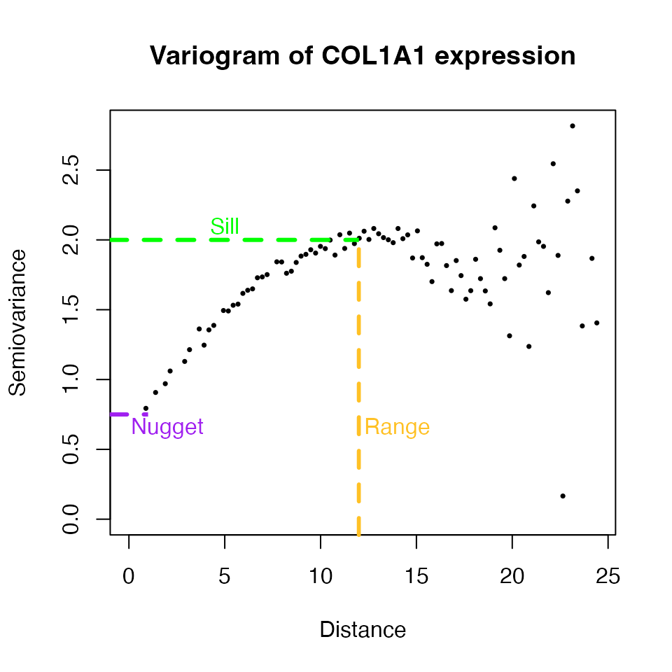

We can see that variance is higher at longer distances. Note, that this relationship is disrupted at longer spot-to-spot distances (> 15 in this case). This disruption occurs because as spot-to-spot distances increase, some spots may belong to distant tissue niches that hold similarity. Regardless, the positive relationship between COL1A1 expression variance and distance is clear a short to medium distances, first increasing and then forming a plateau. Since a relationship exists between COL1A1 expression variance and distance, spatial covariance models defined by the nugget, sill, and range parameters can be fitted to account for spatial dependency.

How is the information in variogram used by STdiff ?

To account for spatial dependency, the STdiff calculates three parameters from the variogram that are necessary to describe the relationship between gene expression variance and distance between spots or cells. The three parameters are known as nugget, sill, and range).

The spatial covariance can be modeled using different covariance structures. The covariance structure that best describes the relationship varies from gene to gene, and from sample to sample. Three popular spatial covariance structures are the exponential, spherical, and gaussian covariance structures, all of them defined in terms of the nugget, sill, and range parameters.

Using the variogram calculated previously, the different covariance structures can be fitted and visualized with geoR like so:

# Exponential covariance structure:
exp_model <- geoR::variofit(vgm, fix.nugget=F, cov.model='exponential',
                            ini.cov.pars=c(0.2, 11), nugget=0.7, # Sill, range, and nugget specified here
                            max.dist=15) # Maximum distance to which model will be fitted
#> variofit: covariance model used is exponential 
#> variofit: weights used: npairs 
#> variofit: minimisation function used: optim

sph_model <- geoR::variofit(vgm, fix.nugget=F, cov.model='spherical',
                            ini.cov.pars=c(0.2, 11), nugget=0.7, 
                            max.dist=15)
#> variofit: covariance model used is spherical 
#> variofit: weights used: npairs 
#> variofit: minimisation function used: optim

gau_model <- geoR::variofit(vgm, fix.nugget=F, cov.model='gaussian',
                            ini.cov.pars=c(0.2, 11), nugget=0.7, 
                            max.dist=15)
#> variofit: covariance model used is gaussian 
#> variofit: weights used: npairs 
#> variofit: minimisation function used: optim

plot(vgm, pch=16, cex=0.5, ylab='Semiovariance', xlab='Distance',
     main=paste0('Variogram of ', gene, ' expression with\nfitted covariance structures'))
text(c(20.5, 20.5, 20.5), c(0.8, 0.6, 0.4), labels=c('Exponential','Spherical', 'Gaussian'))
clip(x1=15, x2=17, y1=-1, y2=2.1)
abline(h=0.8, col=alpha('red', 0.7), lwd=3)
abline(h=0.6, col=alpha('blue', 0.7), lwd=3)
abline(h=0.4, col=alpha('orange', 0.7), lwd=3)
clip(x1=-1, x2=12, y1=-1, y2=2.1)
abline(h=2, col='green', lwd=3, lty=2)
clip(x1=-1, x2=1, y1=-1, y2=2)
abline(h=0.75, col='purple', lwd=3, lty=2)
clip(x1=-1, x2=12.1, y1=-1, y2=2)
abline(v=12, col='goldenrod1', lwd=3, lty=2)
lines(exp_model, col=alpha('red', 0.7), lwd=3)
lines(sph_model, col=alpha('blue', 0.7), lwd=3)
lines(gau_model, col=alpha('orange', 0.7), lwd=3)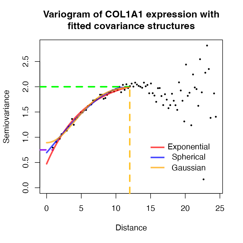

In the case of COL1A1 for sample ‘ST_mel1_rep1’, all models (exponential, spherical, and gaussian) fit well the variogram. Due to computational constraints, the geoR package is not used in spatialGE to estimate the covariance structures. Rather, the spaMM package has been used and only the exponential covariance structure has been implemented. While this choice is not optimal for all genes, accounting for the spatial dependency even if the model fit is not optimal, is likely better than not accounting for the spatial dependency at all.

Differential gene expression analysis with `STdiff`

In addition to Wilcoxon’s rank test and T-test, the STdiff function can also use non-spatial mixed models to test for differentially expressed genes. In the non-spatial mixed models the the expression \(y(s_i)\) of a gene in spot/cell \(i\) is described as:

\[ y(s_i) = μ + ε(s_i) \]

where \(μ\) is the average expression of the gene in the sample, and \(ε(s_i)\) is the random error at spot/cell \(i\).

To reduce the number of false positives in differential expression analysis of ST data, the STdiff function features a novel implementation of spatial mixed models with that expands the non-spatial case to include spatial covariance structures. In the spatial mixed models, the expression \(y(s_i)\) of a gene in spot/cell \(i\) is described as:

\[ Y(s_i) = μ + w(s_i) + ε(s_i) \]

where \(w(s_i)\) denotes the exponential spatial covariance of spot/cell \(i\).

In order to detect differentially expressed genes, groups of spots/cells should be defined first. In the context of ST data, these groups of spots/cells often represent tissue domains. The spatialGE package includes a spatially-informed tissue domain detection method called STclust.

Detection of tissue domains with `STclust`

The STclust function groups spots/cells into tissue domains using hierarchical clustering on a wighted similarity matrix. The similarity maxtrox is derived from Euclidean transcriptomics distances “shrunk” by the spatial Euclidean distances. Please, refer to the journal article describing the method for more details (Ospina et al. 2022). To detect tissue domains, a spatial weight of 0.025 (w=0.025) will be used. The number of domains will be automatically defined by applying dynamicTreeClusters (ks='dtc').

melanoma <- STclust(melanoma, 
                    ks='dtc', 
                    ws=0.025)
#> STclust started.
#> STclust completed in 0.17 min.
#>

Results of STclust domain detection can be plotted using the STplot function:

cluster_p <- STplot(melanoma, 
                    samples='ST_mel1_rep1', 
                    ws=0.025, 
                    deepSplit=F,
                    ptsize=2, color=c('#00BA38', '#619CFF', '#F8766D'))

print(cluster_p[[1]])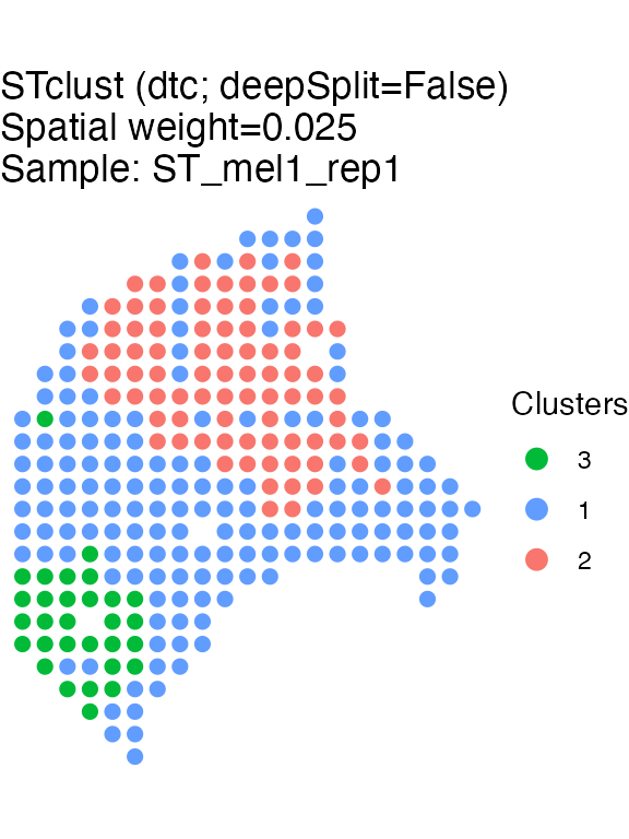

With the domains identified, the STdiff function can be used. The following command tests for differentially expressed genes on the 1000 genes with the highest variation (as defined by Seurat’s function FindVariableFeatures).

deg <- STdiff(melanoma, 
              samples='ST_mel1_rep1', 
              w=0.025, k='dtc', deepSplit=F, 
              topgenes=1000,
              sp_topgenes=0.2) # Test the 20% of the top differtially expressed genes (based on adjusted p-value)
#> Testing STclust assignment (w=0.025, dtc deepSplit=False)...
#>    Running non-spatial mixed models...
#> 
#> Registered S3 methods overwritten by 'registry':
#>   method               from 
#>   print.registry_field proxy
#>   print.registry_entry proxy
#>     Completed non-spatial mixed models (3.59 min).
#>    Running spatial tests...
#> 
#>  Completed spatial mixed models (6.61 min).
#> STdiff completed in 10.25 min.
#>

The output of STdiff is a list, where each element is a data frame containing the test results for each sample:

print(deg[['ST_mel1_rep1']])
#> # A tibble: 3,000 × 9
#>    sample       gene  avg_l…¹ clust…² mm_p_val adj_p_…³ exp_p_…⁴ exp_a…⁵ comme…⁶
#>    <chr>        <chr>   <dbl> <chr>      <dbl>    <dbl>    <dbl>   <dbl> <chr>  
#>  1 ST_mel1_rep1 RP11…  -0.523 1       4.02e-10 6.03e- 9 4.02e-10 1.19e-9 NA     
#>  2 ST_mel1_rep1 PEG10  -0.554 1       6.03e-14 1.64e-12 4.22e-10 1.23e-9 NA     
#>  3 ST_mel1_rep1 RNF44  -0.400 1       4.79e- 8 4.99e- 7 2.77e- 9 6.81e-9 NA     
#>  4 ST_mel1_rep1 ZCCH…  -0.349 1       1.14e- 9 1.54e- 8 7.43e- 9 1.72e-8 NA     
#>  5 ST_mel1_rep1 SHIS…  -0.584 1       1.50e-12 3.21e-11 7.69e- 9 1.76e-8 NA     
#>  6 ST_mel1_rep1 MCOL…  -0.453 1       2.91e-11 5.07e-10 1.23e- 8 2.70e-8 NA     
#>  7 ST_mel1_rep1 TSPA…  -0.853 1       1.20e-14 3.53e-13 1.37e- 8 2.98e-8 NA     
#>  8 ST_mel1_rep1 PPIA   -0.648 1       7.40e-10 1.06e- 8 1.49e- 8 3.21e-8 NA     
#>  9 ST_mel1_rep1 COL1…  -0.527 1       5.89e- 7 4.94e- 6 2.92e- 7 5.73e-7 NA     
#> 10 ST_mel1_rep1 SFRP1  -0.747 1       1.09e- 9 1.47e- 8 6.39e- 7 1.15e-6 NA     
#> # … with 2,990 more rows, and abbreviated variable names ¹avg_log2fc,
#> #   ²cluster_1, ³adj_p_val, ⁴exp_p_val, ⁵exp_adj_p_val, ⁶comments

The columns p_val and adj_p_val are respectively the nominal and adjusted p-values resulting from the differential expression tests using the non-spatial models. The exp_p_val and exp_adj_p_val are the p-values resulting from the spatial models.

Comparing results from the non-spatial and spatial models

We can look at the -log10(p-values) to compare each spatial model to the non-spatial model:

# First load ggrepel to add gene names to plot
library('ggrepel')

# Calculate -log10 p-values
log_pval <- deg[['ST_mel1_rep1']] %>%
  select(gene, cluster_1, mm_p_val, exp_p_val) %>%
  mutate(log_p_val= -log10(mm_p_val+1e-100)) %>% # Add a constant to avoid -log10(0)
  mutate(log_exp_p_val= -log10(exp_p_val+1e-100))

# Create plot
p1 <- ggplot(log_pval, aes(x=log_p_val, y=log_exp_p_val)) +
  geom_abline(intercept=0, slope=1, linetype="dashed") + # Diagonal line... All p-values over this line if equal
  geom_hline(yintercept=-log10(0.05), linetype="dashed", color='gray50') + # Line p-value <0.05
  geom_vline(xintercept=-log10(0.05), linetype="dashed", color='gray50') + # Line p-value <0.05
  geom_point(aes(color=cluster_1)) +
  xlim(0, 20) + ylim(0, 20) + # Restrict axes to ease visualization (very small p-values)
  geom_text_repel(aes(label=gene), size=2, show.legend=F) +
  theme_bw()

p1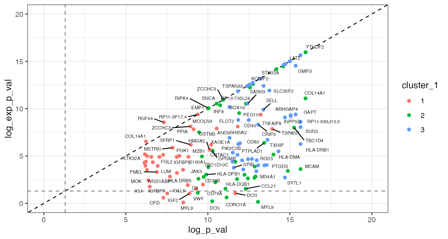

When comparing the -log10(p-values) from the non-spatial and spatial models, it is possible to see that the p-values from the non-spatial model tended to provide smaller, more significant p-values (i.e., larger -log10(p-values), below the 1:1 dotted red line). Some genes such as DCN, MYL9, IGF2 are shown as differentially expressed by the non-spatial models, however, are not differentially expressed in the spatial models (p-values under the -log10(0.05) indicated with horizontal and vertical dashed lines). This pattern is suggestive of type I error inflation.

Testing spatial models with STdiff is both computationally- and time-intensive. The analysis in this tutorial took approximately 18 minutes in a OS machine with a 6-cores Intel Core i7 and 16GB memory. Should the user decide to disable spatial testing, the user only needs to set sp_topgenes=0. When running spatial tests with more genes, and samples assayed with more densely sampled technologies (e.g., Visium, CosMx-SMI), the user should consider running STdiff in a High-Performance Computing environment (HPC, or “cluster”), setting the number of cores to use via the cores parameter.

Does spatialGE support other differential expression test types?

It has been shown above that accounting for spatial dependence between spots/cells is important to control inflation of type-I error (i.e., too many differentially expressed genes). Nonetheless, the STdiff function also implements differential expression analysis using tests commonly used in non-spatial single cell analysis. Specifically, the argument test_type can be set to “wilcoxon” or “t_test” to perform either Wilcoxon’s Rank tests or T-tests respectively:

deg_wilcox <- STdiff(melanoma, 
                     samples='ST_mel1_rep1', 
                     w=0.025, k='dtc', deepSplit=F, 
                     topgenes=1000,
                     test_type='wilcoxon')
#> Testing STclust assignment (w=0.025, dtc deepSplit=False)...
#>    Running Wilcoxon's tests...
#>    Completed Wilcoxon's tests (3.29 min).
#> STdiff completed in 3.29 min.
#>

No spatial tests are executed when Wilcoxon’s Rank tests or T-tests are requested.

print(deg_wilcox[['ST_mel1_rep1']])
#> # A tibble: 3,000 × 6
#>    sample       gene        avg_log2fc cluster_1 wilcox_p_val adj_p_val
#>    <chr>        <chr>            <dbl> <chr>            <dbl>     <dbl>
#>  1 ST_mel1_rep1 PEG10           -0.554 1             4.40e-14  1.20e-12
#>  2 ST_mel1_rep1 COL1A1           1.22  1             1.86e-13  4.44e-12
#>  3 ST_mel1_rep1 MCOLN3          -0.453 1             5.12e-13  1.12e-11
#>  4 ST_mel1_rep1 TSPAN7          -0.853 1             3.57e-12  6.82e-11
#>  5 ST_mel1_rep1 SHISA2          -0.584 1             1.17e-11  2.03e-10
#>  6 ST_mel1_rep1 IGLL5            0.993 1             1.89e-11  3.05e-10
#>  7 ST_mel1_rep1 METRN           -0.560 1             3.59e-11  5.46e-10
#>  8 ST_mel1_rep1 HMGA2           -0.569 1             6.31e-11  9.05e-10
#>  9 ST_mel1_rep1 XAGE1A          -0.581 1             6.35e-11  9.07e-10
#> 10 ST_mel1_rep1 RP11-3P17.4     -0.523 1             8.94e-11  1.22e- 9
#> # … with 2,990 more rows

Visualizng `STdiff` results

The spatialGE package has a built-in function (STdiff_volcano) to generate volcano plots. The function takes STdiff outputs and generates a volcano plot for each sample and cluster (or cluster pair if pairwise testing was requested).

vp <- STdiff_volcano(deg)

Now, the ggpubr package can be used to arrange all plots:

ggpubr::ggarrange(plotlist=vp, ncol=3, common.legend=T)

R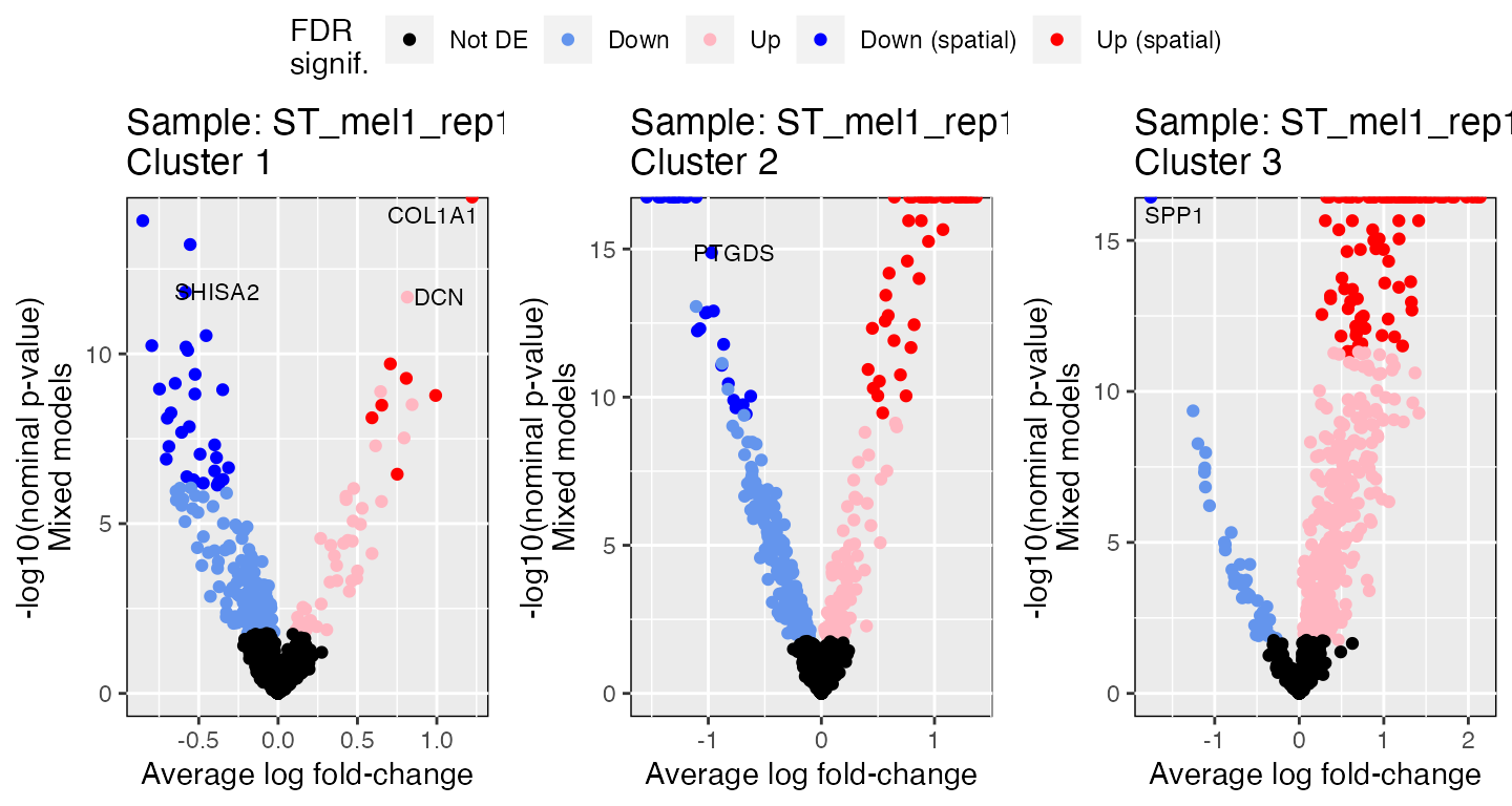eferences

Ospina, Oscar E, Christopher M Wilson, Alex C Soupir, Anders Berglund, Inna Smalley, Kenneth Y Tsai, and Brooke L Fridley. 2022. “spatialGE: quantification and visualization of the tumor microenvironment heterogeneity using spatial transcriptomics.” Bioinformatics 38: 2645–47. https://doi.org/10.1093/bioinformatics/btac145.

Thrane, Kim, Hanna Eriksson, Jonas Maaskola, Johan Hansson, and Joakim Lundeberg. 2018. “Spatially Resolved Transcriptomics Enables Dissection of Genetic Heterogeneity in Stage III Cutaneous Malignant Melanoma.” Cancer Research 78: 5970–79.

Session Info

sessionInfo()
#> R version 4.1.2 (2021-11-01)
#> Platform: x86_64-apple-darwin17.0 (64-bit)
#> Running under: macOS Big Sur 10.16
#> 
#> Matrix products: default
#> BLAS:   /Library/Frameworks/R.framework/Versions/4.1/Resources/lib/libRblas.0.dylib
#> LAPACK: /Library/Frameworks/R.framework/Versions/4.1/Resources/lib/libRlapack.dylib
#> 
#> locale:
#> [1] en_US.UTF-8/en_US.UTF-8/en_US.UTF-8/C/en_US.UTF-8/en_US.UTF-8
#> 
#> attached base packages:
#> [1] stats     graphics  grDevices utils     datasets  methods   base     
#> 
#> other attached packages:
#>  [1] ggrepel_0.9.1   forcats_0.5.1   stringr_1.5.0   dplyr_1.1.0    
#>  [5] purrr_1.0.1     readr_2.1.2     tidyr_1.3.0     tibble_3.2.1   
#>  [9] ggplot2_3.3.5   tidyverse_1.3.1 spatialGE_1.2.0
#> 
#> loaded via a namespace (and not attached):
#>   [1] utf8_1.2.2            reticulate_1.24       tidyselect_1.2.0     
#>   [4] htmlwidgets_1.5.4     grid_4.1.2            Rtsne_0.15           
#>   [7] ggpolypath_0.1.0      munsell_0.5.0         codetools_0.2-18     
#>  [10] ragg_1.2.5            ica_1.0-2             future_1.23.0        
#>  [13] miniUI_0.1.1.1        withr_2.5.0           colorspace_2.0-2     
#>  [16] highr_0.9             knitr_1.37            rstudioapi_0.13      
#>  [19] Seurat_4.1.0          ROCR_1.0-11           ggsignif_0.6.3       
#>  [22] tensor_1.5            listenv_0.8.0         labeling_0.4.2       
#>  [25] slam_0.1-50           splancs_2.01-42       polyclip_1.10-0      
#>  [28] bit64_4.0.5           farver_2.1.0          rprojroot_2.0.2      
#>  [31] parallelly_1.30.0     vctrs_0.6.2           generics_0.1.2       
#>  [34] xfun_0.31             R6_2.5.1              khroma_1.8.0         
#>  [37] fields_14.1           spatstat.utils_3.0-1  cachem_1.0.6         
#>  [40] assertthat_0.2.1      promises_1.2.0.1      scales_1.2.0         
#>  [43] vroom_1.5.7           gtable_0.3.0          globals_0.14.0       
#>  [46] goftest_1.2-3         spam_2.9-1            rlang_1.1.1          
#>  [49] systemfonts_1.0.4     splines_4.1.2         rstatix_0.7.0        
#>  [52] lazyeval_0.2.2        spatstat.geom_3.0-6   broom_0.7.12         
#>  [55] yaml_2.2.2            reshape2_1.4.4        abind_1.4-5          
#>  [58] modelr_0.1.8          backports_1.4.1       httpuv_1.6.5         
#>  [61] tools_4.1.2           tcltk_4.1.2           ellipsis_0.3.2       
#>  [64] spatstat.core_2.3-2   jquerylib_0.1.4       geoR_1.9-2           
#>  [67] RColorBrewer_1.1-2    proxy_0.4-26          dynamicTreeCut_1.63-1
#>  [70] wordspace_0.2-6       ggridges_0.5.3        Rcpp_1.0.10          
#>  [73] plyr_1.8.6            spaMM_4.2.1           ggpubr_0.4.0         
#>  [76] rpart_4.1-15          deldir_1.0-6          pbapply_1.5-0        
#>  [79] viridis_0.6.2         cowplot_1.1.1         ROI_1.0-0            
#>  [82] zoo_1.8-9             SeuratObject_4.0.4    haven_2.4.3          
#>  [85] cluster_2.1.2         fs_1.5.2              magrittr_2.0.2       
#>  [88] data.table_1.14.2     scattermore_0.7       lmtest_0.9-39        
#>  [91] reprex_2.0.1          RANN_2.6.1            fitdistrplus_1.1-6   
#>  [94] matrixStats_0.61.0    hms_1.1.1             patchwork_1.1.1      
#>  [97] mime_0.12             evaluate_0.14         xtable_1.8-4         
#> [100] sparsesvd_0.2         readxl_1.3.1          gridExtra_2.3        
#> [103] compiler_4.1.2        maps_3.4.0            KernSmooth_2.23-20   
#> [106] crayon_1.4.2          minqa_1.2.4           htmltools_0.5.2      
#> [109] mgcv_1.8-38           later_1.3.0           tzdb_0.3.0           
#> [112] lubridate_1.8.0       DBI_1.1.2             dbplyr_2.1.1         
#> [115] MASS_7.3-54           boot_1.3-28           car_3.0-12           
#> [118] Matrix_1.4-1          cli_3.6.0             parallel_4.1.2       
#> [121] dotCall64_1.0-1       igraph_1.2.11         pkgconfig_2.0.3      
#> [124] pkgdown_2.0.7         registry_0.5-1        numDeriv_2016.8-1.1  
#> [127] sp_1.4-6              plotly_4.10.0         spatstat.sparse_3.0-0
#> [130] xml2_1.3.3            bslib_0.3.1           iotools_0.3-2        
#> [133] rvest_1.0.2           digest_0.6.29         sctransform_0.3.3    
#> [136] RcppAnnoy_0.0.19      spatstat.data_3.0-0   rmarkdown_2.14       
#> [139] cellranger_1.1.0      leiden_0.3.9          uwot_0.1.11          
#> [142] shiny_1.7.1           nloptr_2.0.0          lifecycle_1.0.3      
#> [145] nlme_3.1-153          jsonlite_1.7.3        carData_3.0-5        
#> [148] desc_1.4.2            viridisLite_0.4.0     fansi_1.0.2          
#> [151] pillar_1.8.1          lattice_0.20-45       fastmap_1.1.0        
#> [154] httr_1.4.2            survival_3.4-0        glue_1.6.2           
#> [157] png_0.1-7             bit_4.0.4             stringi_1.7.6        
#> [160] sass_0.4.0            textshaping_0.3.6     memoise_2.0.1        
#> [163] irlba_2.3.5           future.apply_1.8.1

2023-09-02