This will be a short vignette for using all of the functions that derives spatial metrics
library(spatialTIME)
#> spatialTIME version:
#> 1.3.4.1
#> If using for publication, please cite our manuscript:
#> https://doi.org/10.1093/bioinformatics/btab757
library(tidyverse)
Create mIF object
mif = create_mif(clinical_data = example_clinical %>%
                   mutate(deidentified_id = as.character(deidentified_id)),
                 sample_data = example_summary %>%
                   mutate(deidentified_id = as.character(deidentified_id)),
                 spatial_list = example_spatial,
                 patient_id = "deidentified_id",
                 sample_id = "deidentified_sample")
mif
#> 229 patients spanning 229 samples and 5 spatial data frames were foundRipley’s K
Univariate
mif = ripleys_k(mif = mif,
                mnames = markers[1:2],
                r_range = 0:100,
                num_permutations = 50,
                edge_correction = "translation",
                permute = TRUE,
                keep_permutation_distribution = FALSE,
                workers = 1,
                overwrite = TRUE,
                xloc = NULL,
                yloc = NULL)

mif$derived$univariate_Count %>%
  ggplot() +
  geom_line(aes(x = r, y = `Degree of Clustering Permutation`, color = deidentified_sample)) +
  facet_grid(~Marker)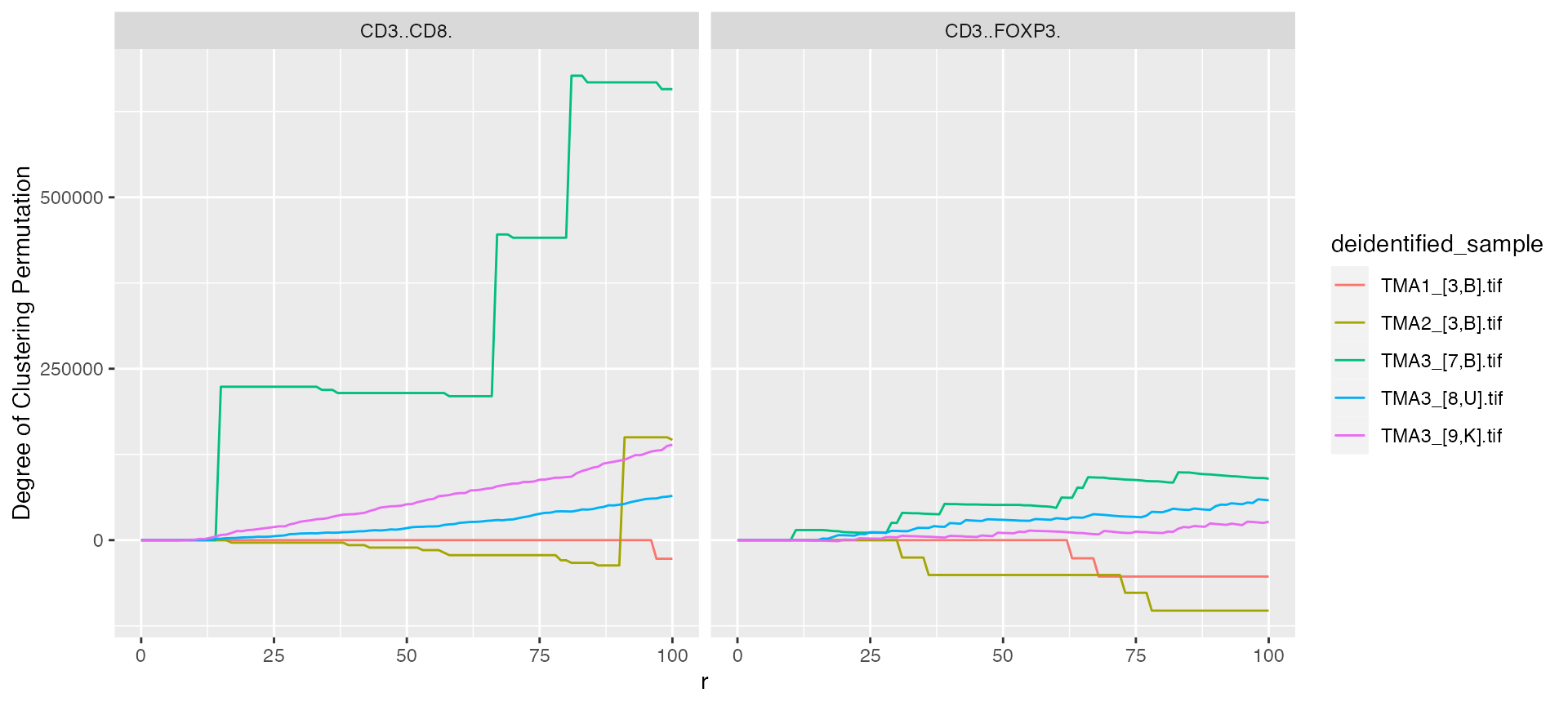
Bivariate
mif = bi_ripleys_k(mif = mif,
                   mnames = markers[1:2],
                   r_range = 0:100,
                   num_permutations = 50,
                   edge_correction = "translation",
                   permute = TRUE,
                   keep_permutation_distribution = FALSE,
                   workers = 1,
                   overwrite = TRUE,
                   xloc = NULL,
                   yloc = NULL)

mif$derived$bivariate_Count %>%
  ggplot() +
  geom_line(aes(x = r, y = `Degree of Clustering Permutation`, color = deidentified_sample)) +
  facet_grid(~Anchor)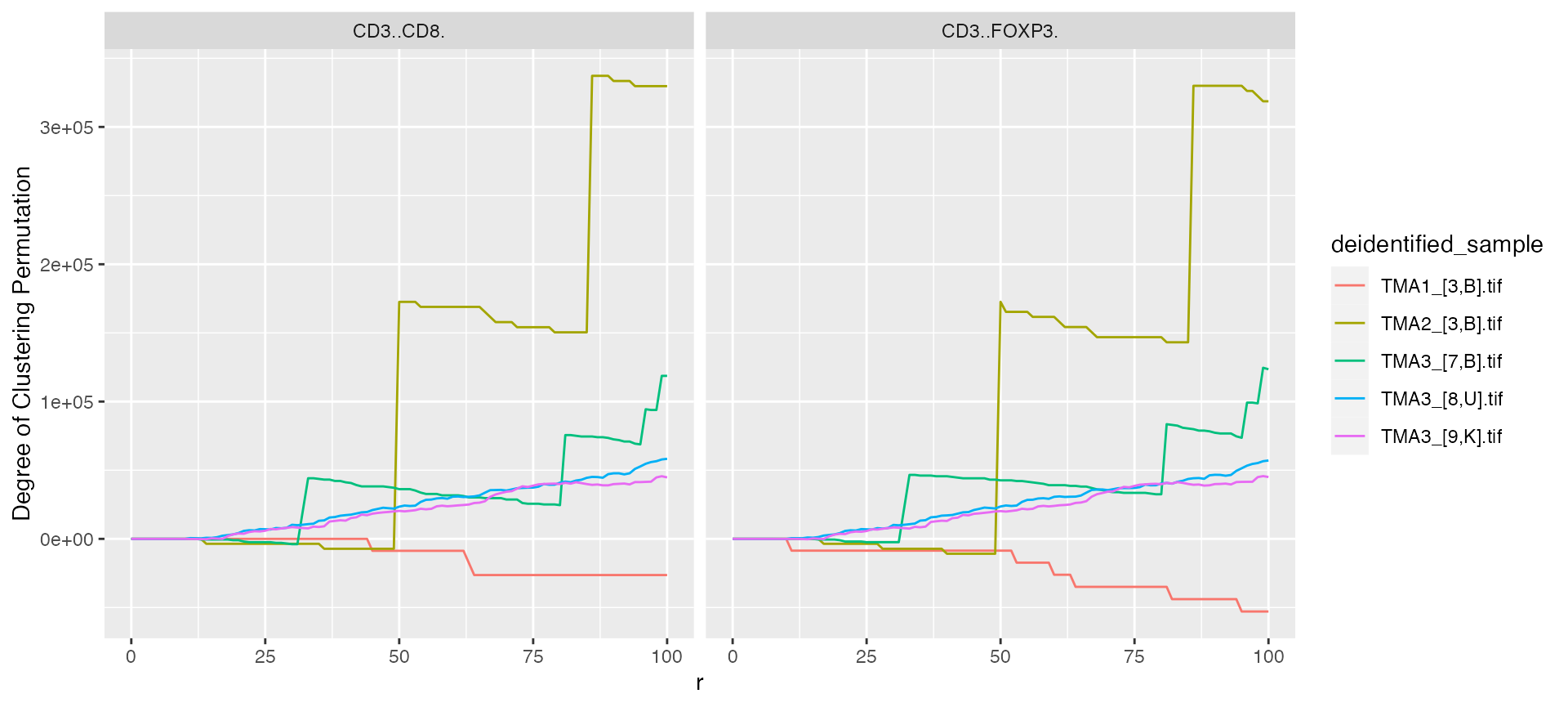
Nearest Neighbor G
Univariate
mif = NN_G(mif = mif,
           mnames = markers[1:2],
           r_range = 0:100,
           num_permutations = 50,
           edge_correction = "rs",
           keep_perm_dis = FALSE,
           workers = 1,
           overwrite = TRUE,
           xloc = NULL,
           yloc = NULL)

mif$derived$univariate_NN %>%
  ggplot() +
  geom_line(aes(x = r, y = `Degree of Clustering Permutation`, color = deidentified_sample)) +
  facet_grid(~Marker)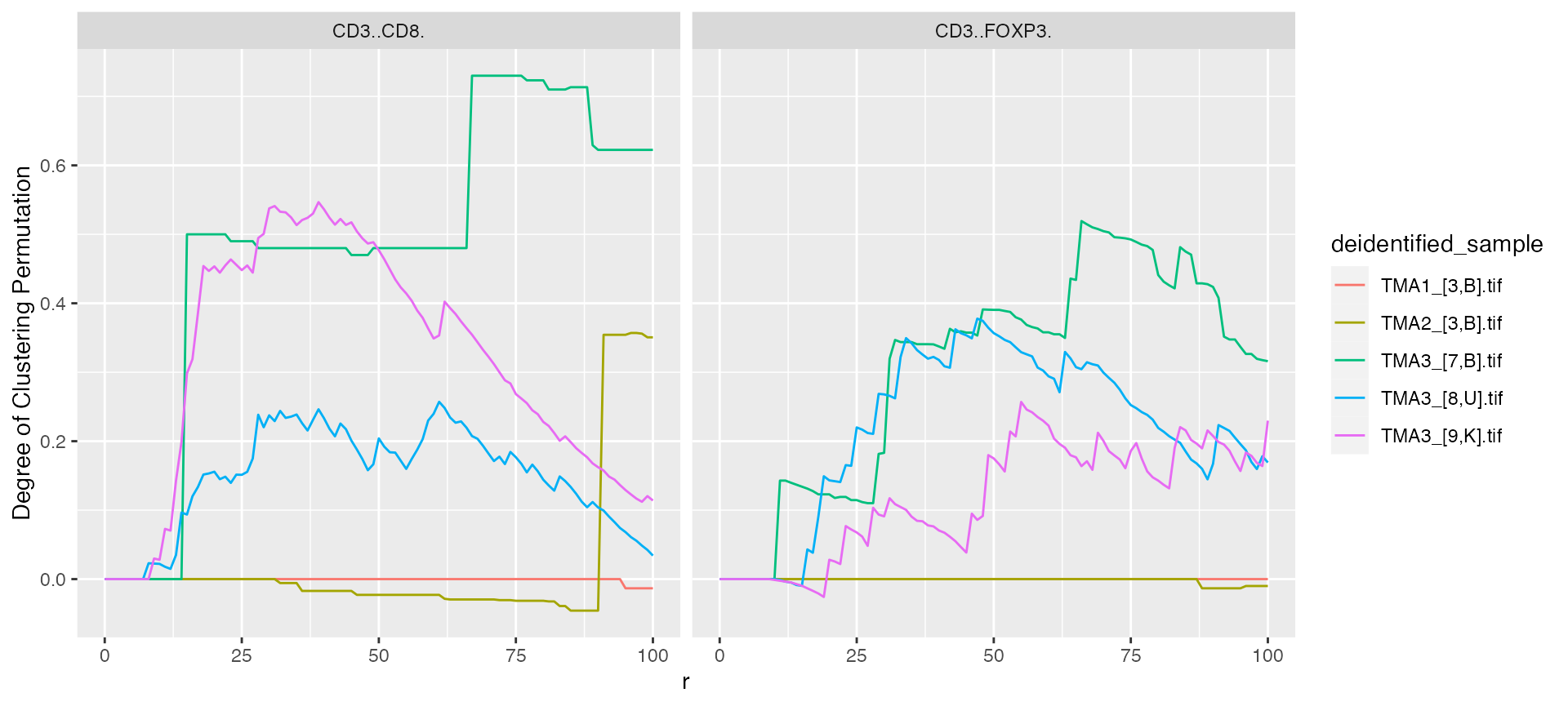
Bivariate
mif = bi_NN_G(mif = mif,
           mnames = markers[1:2],
           r_range = 0:100,
           num_permutations = 50,
           edge_correction = "rs",
           keep_perm_dis = FALSE,
           workers = 1,
           overwrite = TRUE,
           xloc = NULL,
           yloc = NULL)

mif$derived$bivariate_NN %>%
  ggplot() +
  geom_line(aes(x = r, y = `Degree of Clustering Permutation`, color = deidentified_sample)) +
  facet_grid(~Anchor)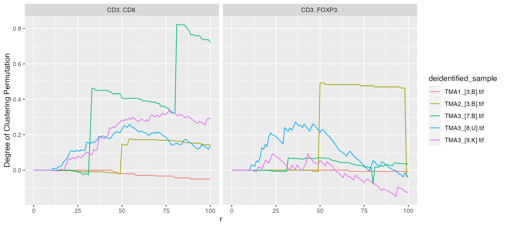
Pair Correlation g
Univariate
mif = pair_correlation(mif = mif,
                       mnames = markers[1:2],
                       r_range = 0:100,
                       num_permutations = 50,
                       edge_correction = "translation",
                       keep_permutation_distribution = FALSE,
                       workers = 1,
                       overwrite = TRUE,
                       xloc = NULL,
                       yloc = NULL)

mif$derived$univariate_pair_correlation %>%
  ggplot() +
  geom_line(aes(x = r, y = `Degree of Correlation Permuted`, color = deidentified_sample)) +
  facet_grid(~Marker)
#> Warning: Removed 5 rows containing missing values (`geom_line()`).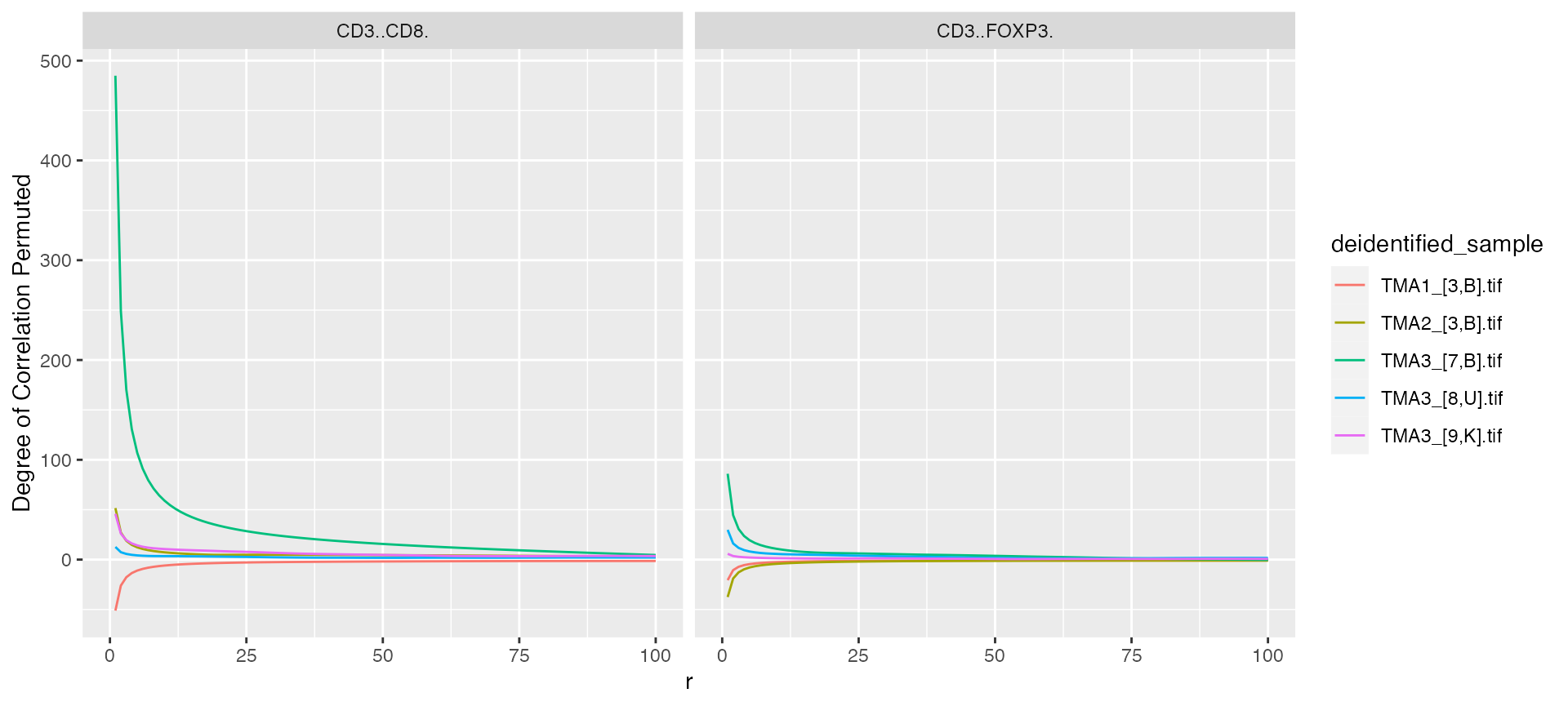
Bivariate
mif = bi_pair_correlation(mif = mif,
                       mnames = markers[1:2],
                       r_range = 0:100,
                       num_permutations = 50,
                       edge_correction = "translation",
                       keep_permutation_distribution = FALSE,
                       workers = 1,
                       overwrite = TRUE,
                       xloc = NULL,
                       yloc = NULL)

mif$derived$bivariate_pair_correlation %>%
  ggplot() +
  geom_line(aes(x = r, y = `Degree of Correlation Permuted`, color = deidentified_sample)) +
  facet_grid(~From)
#> Warning: Removed 5 rows containing missing values (`geom_line()`).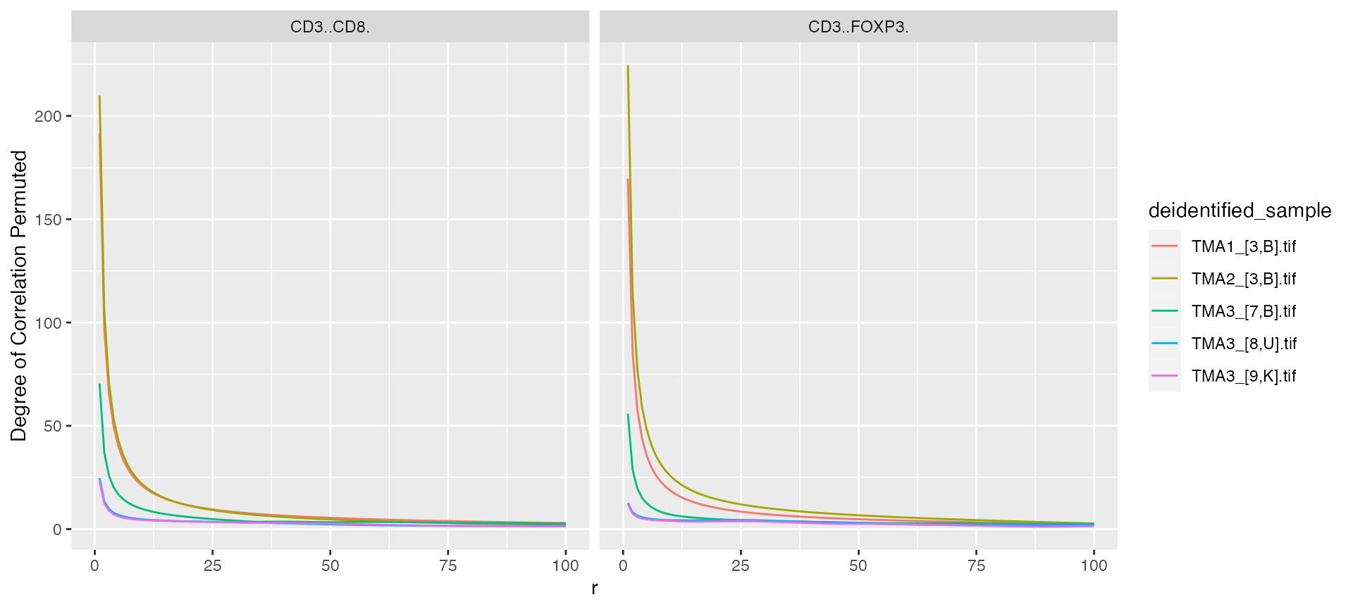
Interaction Variable
mif = interaction_variable(mif = mif,
                           mnames = markers[1:2],
                           r_range = 0:100,
                           num_permutations = 50,
                           keep_permutation_distribution = FALSE,
                           workers = 1,
                           overwrite = TRUE,
                           xloc = NULL,
                           yloc = NULL)

mif$derived$interaction_variable %>%
  ggplot() +
  geom_line(aes(x = r, y = `Degree of Interaction Permuted`, color = deidentified_sample)) +
  facet_grid(~From)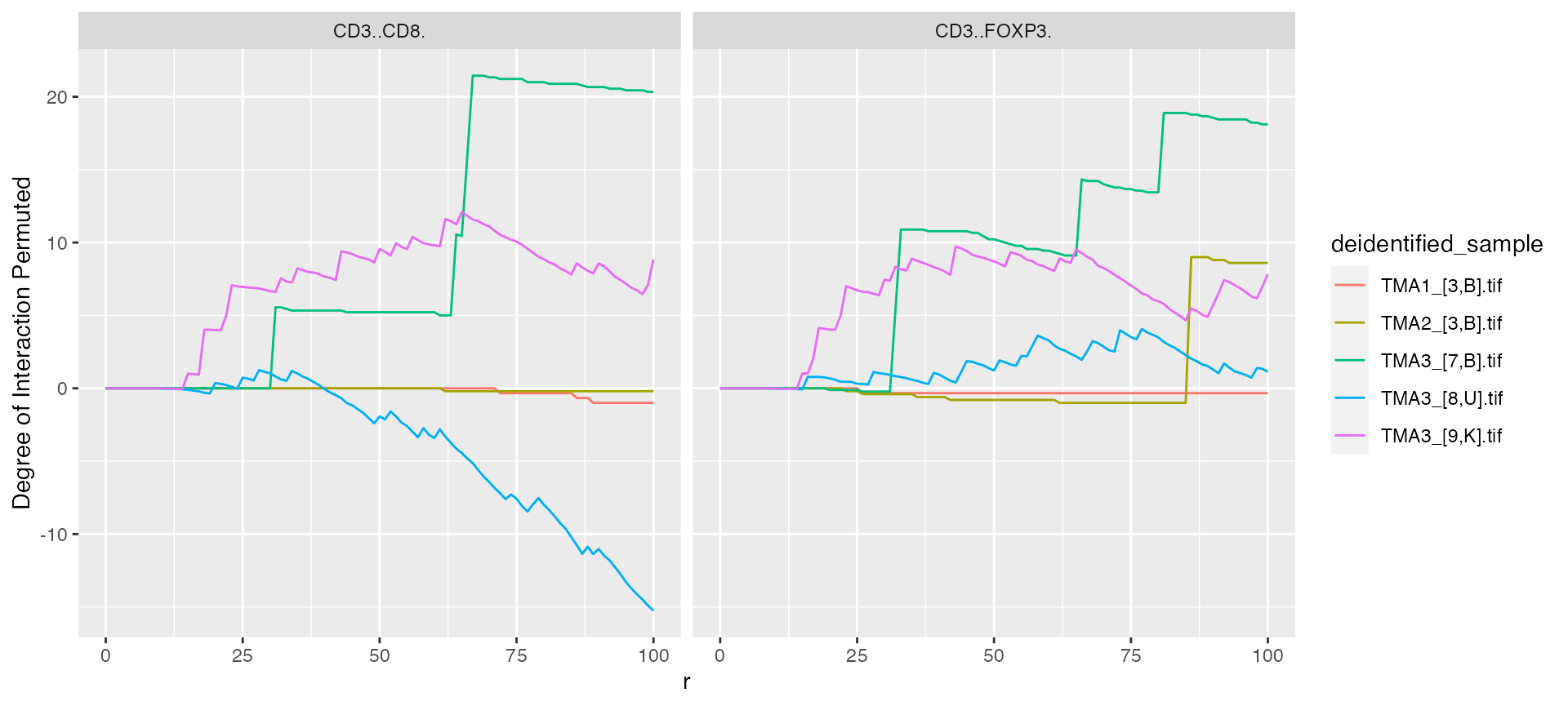
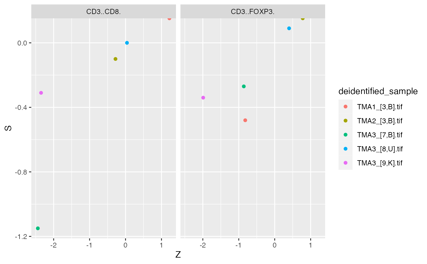
Dixon’s Segregation S
mif = dixons_s(mif = mif,
               mnames = markers[1:2],
               num_permutations = 50,
               type = "Z",
               workers = 1,
               overwrite = TRUE,
               xloc = NULL,
               yloc = NULL)
#> The legacy packages maptools, rgdal, and rgeos, underpinning the sp package,
#> which was just loaded, will retire in October 2023.
#> Please refer to R-spatial evolution reports for details, especially
#> https://r-spatial.org/r/2023/05/15/evolution4.html.
#> It may be desirable to make the sf package available;
#> package maintainers should consider adding sf to Suggests:.
#> The sp package is now running under evolution status 2
#>      (status 2 uses the sf package in place of rgdal)
#> 1, 2, 3, 4, 5, 6, 7, 8, 9, 10, 11, 12, 13, 14, 15, 16, 17, 18, 19, 20,
#> 21, 22, 23, 24, 25, 26, 27, 28, 29, 30, 31, 32, 33, 34, 35, 36, 37, 38, 39, 40,
#> 41, 42, 43, 44, 45, 46, 47, 48, 49,
#> 50.
#> 1, 2, 3, 4, 5, 6, 7, 8, 9, 10, 11, 12, 13, 14, 15, 16, 17, 18, 19, 20,
#> 21, 22, 23, 24, 25, 26, 27, 28, 29, 30, 31, 32, 33, 34, 35, 36, 37, 38, 39, 40,
#> 41, 42, 43, 44, 45, 46, 47, 48, 49,
#> 50.
#> 1, 2, 3, 4, 5, 6, 7, 8, 9, 10, 11, 12, 13, 14, 15, 16, 17, 18, 19, 20,
#> 21, 22, 23, 24, 25, 26, 27, 28, 29, 30, 31, 32, 33, 34, 35, 36, 37, 38, 39, 40,
#> 41, 42, 43, 44, 45, 46, 47, 48, 49,
#> 50.
#> 1, 2, 3, 4, 5, 6, 7, 8, 9, 10, 11, 12, 13, 14, 15, 16, 17, 18, 19, 20,
#> 21, 22, 23, 24, 25, 26, 27, 28, 29, 30, 31, 32, 33, 34, 35, 36, 37, 38, 39, 40,
#> 41, 42, 43, 44, 45, 46, 47, 48, 49,
#> 50.
#> 1, 2, 3, 4, 5, 6, 7, 8, 9, 10, 11, 12, 13, 14, 15, 16, 17, 18, 19, 20,
#> 21, 22, 23, 24, 25, 26, 27, 28, 29, 30, 31, 32, 33, 34, 35, 36, 37, 38, 39, 40,
#> 41, 42, 43, 44, 45, 46, 47, 48, 49,
#> 50.

mif$derived$Dixon_Z %>%
    filter(From != To) %>%
    ggplot() +
    geom_point(aes(x = Z, y = S, color = deidentified_sample)) +
    facet_grid(~From)